– 의류 이미지 분류 (Fashion MNIST)
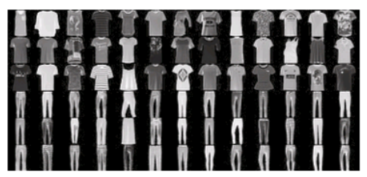
– 의류 데이터 준비
※ TensorFlow 최신 버전 설치
!pip install tensorflow_gpu==2.6.0
1. TensorFlow 가져오기
import tensorflow as tf
2. TensorFlow 버전 확인
tf.__version__


##출력: '2.6.0'
3. 모드 MNIST 레코드 로드
(x_train_all, y_train_all), (x_test, y_test) = tf.keras.datasets.fashion_mnist.load_data()
4. 훈련 세트의 크기 확인
print(x_train_all.shape, y_train_all.shape)


##출력: (60000, 28, 28) (60000,)

5. imshow() 함수를 사용하여 샘플 이미지 확인
import matplotlib.pyplot as plt

plt.imshow(x_train_all(0), cmap='gray')
plt.show()
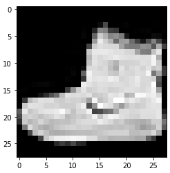
6. 목표의 내용과 중요성 검토
print(y_train_all(:10))


##출력: (9 0 0 3 0 2 7 2 5 5)
7. 목표 분포 확인
class_names = ('티셔츠/윗도리', '바지', '스웨터', '드레스', '코트', '샌들', '셔츠', '스니커즈', '가방', '앵클부츠')

print(class_names(y_train_all(0)))


##출력 : 앵클부츠
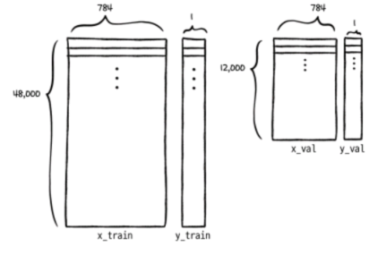
8. 교육 및 검증 세트를 균등하게 분할
from sklearn.model_selection import train_test_split

x_train, x_val, y_train, y_val = train_test_split(x_train_all, y_train_all, stratify=y_train_all, test_size=0.2, random_state=42)
9. 입력 데이터 정규화
x_train = x_train / 255
x_val = x_val / 255
10. 학습 세트 및 검증 세트의 차원 수정
x_train = x_train.reshape(-1, 784)
x_val = x_val.reshape(-1, 784)

print(x_train.shape, x_val.shape)


##출력: (48000, 784) (12000, 784)
반응형
– 멀티클래스 분류를 위한 목표 데이터 준비 및 신경망 훈련
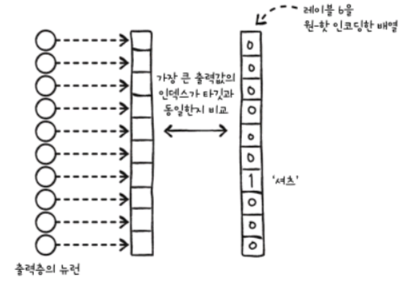
1. 대상을 원-핫 인코딩으로 변환
from sklearn.preprocessing import LabelBinarizer
lb = LabelBinarizer()
lb.fit_transform((0, 1, 3, 1))


##출력:
array(((1, 0, 0),
       (0, 1, 0),
       (0, 0, 1),
       (0, 1, 0)))

2. 배열의 각 요소를 뉴런의 출력과 비교합니다.
tf.keras.utils.to_categorical((0, 1, 3))


##출력:
array(((1., 0., 0., 0.),
       (0., 1., 0., 0.),
       (0., 0., 0., 1.)), dtype=float32)
3. to_categorical 함수를 이용한 원-핫 코딩
y_train_encoded = tf.keras.utils.to_categorical(y_train)
y_val_encoded = tf.keras.utils.to_categorical(y_val)

print(y_train_encoded.shape, y_val_encoded.shape)


##출력: (48000, 10) (12000, 10)

print(y_train(0), y_train_encoded(0))


##출력: 6 (0. 0. 0. 0. 0. 0. 1. 0. 0. 0.)
4. MultiClassNetwork 클래스로 다중 분류 신경망 훈련
fc = MultiClassNetwork(units=100, batch_size=256)
fc.fit(x_train, y_train_encoded, x_val=x_val, y_val=y_val_encoded, epochs=40)
5. 훈련 손실, 검증 손실 도표 및 훈련 모델 점수 검토
plt.plot(fc.losses)
plt.plot(fc.val_losses)
plt.ylabel('loss')
plt.xlabel('iteration')
plt.legend(('train_loss', 'val_loss'))
plt.show()
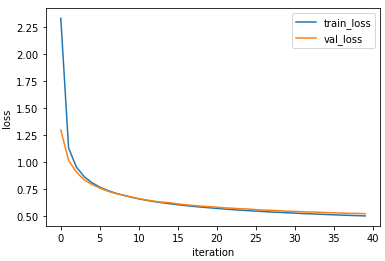
fc.score(x_val, y_val_encoded)

##출력: 0.8150833333333334


np.random.permutation(np.arange(12000)%10)

##출력: array((4, 6, 3, ..., 0, 6, 6))


np.sum(y_val == np.random.permutation(np.arange(12000)%10)) / 12000

##출력: 0.10325
※ 내용